Finding & Downloading Data
Required R Packages & Preparations
First, we install and load relevant packages to our R session. You will see that I do this in a bit of a peculiar fashion. Why do I do this with a custom function as seen below instead of using the lirbary() function in R? I want my scripts to be transferrable across systems (e.g., different computers I work on) and installations of R. SOme of those have the packages I need installed while others don’t. The function I coded below called install.load.package() takes the name of an R package, checks if it is installed and installs it if it isn’t. Subsequently, the function loads the package in question. By applying this function to a vector of package names, we can easily load all packages we need without needing to also run installation functions or accidently overriding an existing installation.
For this part of the tutorial, we need these packages:
## Custom install & load function
install.load.package <- function(x) {
  if (!require(x, character.only = TRUE)) {
    install.packages(x, repos = "http://cran.us.r-project.org")
  }
  require(x, character.only = TRUE)
}
## names of packages we want installed (if not installed yet) and loaded
package_vec <- c(
  "rgbif", # for access to gbif
  "knitr" # for rmarkdown table visualisations
)
## executing install & load for each package
sapply(package_vec, install.load.package)
## rgbif knitr
##  TRUE  TRUE
R as demonstrated in the setup section.
Study Characteristics
To make these exercises more tangible to you, I will walk you through a mock-study within which we will find relevant GBIF-mediated data, download this data, load it into R and clean it, and finally join it with relevant abiotic data ready for a subseqeuent analysis or species distribution modelling exercise (a common use-case of GBIF-mediated data).
Organisms
Let’s first focus on our organisms of interest: conifers and beeches. Why these two? For a few reasons, mainly:
- These are sessile organisms which lend themselves well to species distribution modelling
- These are long-lived species which lend themselves well to species distribution modelling and it use of climate data across long time-scales
- We are all familiar with at least some of these species.
- I think they are neat. They form the backdrop for a lot of wonderful hikes for me - just look at them:

Area
Looking at the world at once, while often something that macroecologists strive for, is unfeasible for our little seasonal school. Consequently, we need to limit our area-of-study to a relevant and familiar region to us. Since the seasonal school is organised within Germany, I assume that Germany would be a good study region for us. Plus, we know we have conifers and beeches there.
Timeframe
Lastly, we need to settle on a timeframe at which to investigate our study organisms in their environments - let’s choose a large time-window to align with the fact that our species of interest live long and to demonstrate some neat functionality of retrieving non-standard environment data later: 1970 to 2020 should be fine!
Finding Data with rgbif
We’ve got our study organisms, we know when and where to look for them - now how can GBIF help us find relevant data?
Resolving Taxonomic Names
First, we need to identify the backbone key by which GBIF indexes data for conifers and beeches. To do so, we make use of the binomial nomenclature frequently used in taxanomy and search for Pinaceae and Fagaceae (conifers and beeches, respectively) within the GBIF backbone taxonomy. We do so with the name_backbone() function:
Pinaceae_backbone <- name_backbone(name = "Pinaceae")
knitr::kable(Pinaceae_backbone) # I do this here for a nice table output in the html page you are looking at
| usageKey | scientificName | canonicalName | rank | status | confidence | matchType | kingdom | phylum | order | family | kingdomKey | phylumKey | classKey | orderKey | familyKey | synonym | class | verbatim_name |
|---|---|---|---|---|---|---|---|---|---|---|---|---|---|---|---|---|---|---|
| 3925 | Pinaceae | Pinaceae | FAMILY | ACCEPTED | 96 | EXACT | Plantae | Tracheophyta | Pinales | Pinaceae | 6 | 7707728 | 194 | 640 | 3925 | FALSE | Pinopsida | Pinaceae |
Pinaceae_key <- Pinaceae_backbone$familyKey

Fagaceae_backbone <- name_backbone(name = "Fagaceae")
knitr::kable(Fagaceae_backbone) # I do this here for a nice table output in the html page you are looking at
| usageKey | scientificName | canonicalName | rank | status | confidence | matchType | kingdom | phylum | order | family | kingdomKey | phylumKey | classKey | orderKey | familyKey | synonym | class | verbatim_name |
|---|---|---|---|---|---|---|---|---|---|---|---|---|---|---|---|---|---|---|
| 4689 | Fagaceae | Fagaceae | FAMILY | ACCEPTED | 96 | EXACT | Plantae | Tracheophyta | Fagales | Fagaceae | 6 | 7707728 | 220 | 1354 | 4689 | FALSE | Magnoliopsida | Fagaceae |
Fagaceae_key <- Fagaceae_backbone$familyKey
Data Discovery
How do we know if GBIF even mediates any data for the taxonomic families we are interested in within our study area across our time frame of interest? Well, we could query a download from GBIF, however, doing so takes time. Alternatively, we can use the occ_search() or occ_count() functions to get a much, much faster overview of data availability. Since occ_search() is very inviting to adopt it for sub-optimal data download practices, let’s focus on occ_count() for now and forget the other functione even exists (personally, I have never found a reason to use occ_search() over occ_count() for the purpose of data discovery).
Let’s build the data discovery call stepp by step for Pinaceae and then apply the same to the Fagaceae:
- How many observations does GBIF mediate for Pinaceae?
occ_count(familyKey = Pinaceae_key)
## [1] 4958280
- How many observations does GBIF mediate for Pinaceae in Germany?
occ_count(
  familyKey = Pinaceae_key,
  country = "DE" # ISO 3166-1 alpha-2 country code
)
## [1] 313109
- How many observations does GBIF mediate for Pinaceae in Germany between 1970 and 2020?
occ_count(
  familyKey = Pinaceae_key,
  country = "DE",
  year = "1970,2020" # year-span identified by comma between start- and end-year
)
## [1] 238098
occ_count() is a good place to start looking for those.
Finally, let’s look at how much data we can obtain for Fagaceae and also for Pinaceae and Fagaceae at the same time:
occ_count(
  familyKey = Fagaceae_key,
  country = "DE",
  year = "1970,2020"
)
## [1] 230461
occ_count(
  familyKey = paste(Fagaceae_key, Pinaceae_key, sep = ";"), # multiple entries that don't indicate a span or series are separated with a semicolon
  country = "DE",
  year = "1970,2020"
)
## [1] 468559
Who would have thought? If we add the number of observations available for Pinaceae and those available for Fagaceae, we get the number of observation available for Pinaceae and Fagaceae.
Downloading Data with rgbif
Toensure reproducibility and data richness of our downloads, we must make a formal download query to the GBIF API and await processing of our data request - an asynchronous download. To do so, we need to do three things in order:
- Specify the data we want and request processing and download from GBIF
- Download the data once it is processed
- Load the downloaded data into
R
Let’s tackle these step-by-step.
Data Request at GBIF
To start this process of obtaining GBIF-mediated occurrence records, we first need to make a request to GBIF to start processing of the data we require. This is done with the occ_download(...) function. Making a data request at GBIF via the occ_download(...) function comes with two important considerations:
occ_download(...)specific syntax- data query metadata
Syntax and Query through occ_download()
The occ_download(...) function - while powerful - requires us to confront a new set of syntax which translates the download request as we have seen it so far into a form which the GBIF API can understand. To do so, we use a host of rgbif functions built around the GBIF predicate DSL (domain specific language). These functions (with a few exceptions which you can see by calling the documentation - ?download_predicate_dsl) all take two arguments:
key- this is a core term which we want to target for our requestvalue- this is the value for the core term which we are interested in
Finally, the relevant functions and how the relate key to value are:
pred(...): equalspred_lt(...): lessThanpred_lte(...): lessThanOrEqualspred_gt(...): greaterThanpred_gte(...): greaterThanOrEqualspred_like(...): likepred_within(...): within (only for geospatial queries, and only accepts a WKT string)pred_notnull(...): isNotNull (only for geospatial queries, and only accepts a WKT string)pred_isnull(...): isNull (only for stating that you want a key to be null)pred_and(...): and (accepts multiple individual predicates, separating them by either “and” or “or”)pred_or(...): or (accepts multiple individual predicates, separating them by either “and” or “or”)pred_not(...): not (negates whatever predicate is passed in)pred_in(...): in (accepts a single key but many values; stating that you want to search for all the values)
Let us use these to query the data we are interested in and add a new parameter into our considerations - we only want human observations of our trees:
res <- occ_download(
  pred_or(
    pred("taxonKey", Pinaceae_key),
    pred("taxonKey", Fagaceae_key)
  ),
  pred("basisOfRecord", "HUMAN_OBSERVATION"),
  pred("country", "DE"),
  pred_gte("year", 1970),
  pred_lte("year", 2020)
)
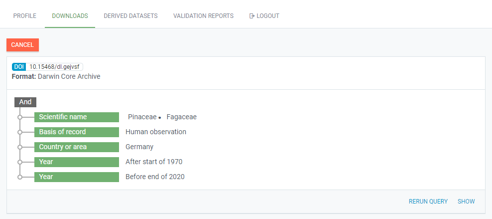
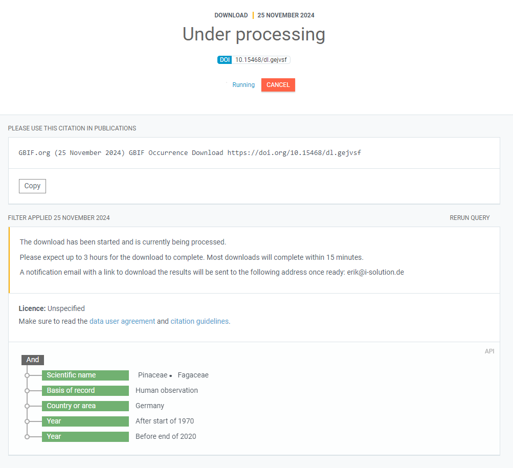
If you navigate to your downloads tab on the GBIF website, you should now see the data request being processed:

You can expand this view request to get more information:

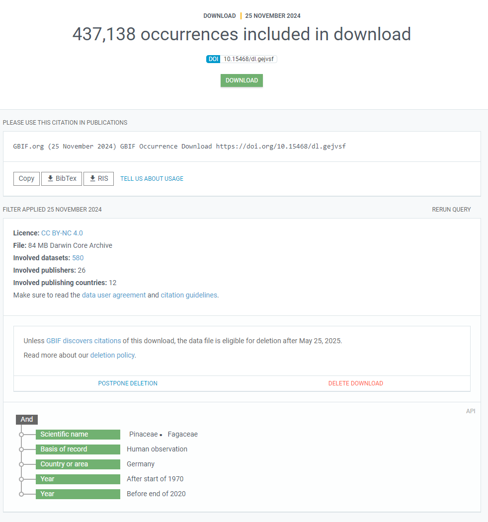
Finally, when the data request is processed and ready for download, you will receive an E-mail telling you so and the view of the request on the webpage will change:

R do the waiting for you.
Downloading Requested Data
Instead of waiting for the confirmation that our query has been processed, let’s just use an rgbif function to do the waiting for us and then continue on to download the processed data once it is ready:
## Check GBIF whether data is ready, this function will finish running when done and return metadata
res_meta <- occ_download_wait(res, status_ping = 10, quiet = FALSE)
## Download the data as .zip (can specify a path)
res_get <- occ_download_get(res)
Loading Downloaded Data into R & Saving Data
All that is left to do is to load the data we just downloaded into R, reformat it, and save it to our hard drive in a format that is easier to load and use with R and other software further down the line:
## Load the data into R
res_data <- occ_download_import(res_get)
write.csv(res_data, file = "NFDI4Bio_GBIF.csv")
For the sake of reproducibility, I would always recommend you also save the GBIF query object. We will use this when discussing citing data download via GBIF.
save(res, file = "NFDI4Bio_GBIF.RData")
Session Info
## R version 4.4.0 (2024-04-24 ucrt)
## Platform: x86_64-w64-mingw32/x64
## Running under: Windows 11 x64 (build 22631)
##
## Matrix products: default
##
##
## locale:
## [1] LC_COLLATE=Norwegian Bokmål_Norway.utf8  LC_CTYPE=Norwegian Bokmål_Norway.utf8
## [3] LC_MONETARY=Norwegian Bokmål_Norway.utf8 LC_NUMERIC=C
## [5] LC_TIME=Norwegian Bokmål_Norway.utf8
##
## time zone: Europe/Oslo
## tzcode source: internal
##
## attached base packages:
## [1] stats     graphics  grDevices utils     datasets  methods   base
##
## other attached packages:
## [1] knitr_1.48  rgbif_3.8.1
##
## loaded via a namespace (and not attached):
##  [1] styler_1.10.3     sass_0.4.9        utf8_1.2.4        generics_0.1.3
##  [5] xml2_1.3.6        blogdown_1.19     stringi_1.8.4     httpcode_0.3.0
##  [9] digest_0.6.37     magrittr_2.0.3    evaluate_0.24.0   grid_4.4.0
## [13] bookdown_0.40     fastmap_1.2.0     R.oo_1.26.0       R.cache_0.16.0
## [17] plyr_1.8.9        jsonlite_1.8.8    R.utils_2.12.3    whisker_0.4.1
## [21] crul_1.5.0        urltools_1.7.3    httr_1.4.7        purrr_1.0.2
## [25] fansi_1.0.6       scales_1.3.0      oai_0.4.0         lazyeval_0.2.2
## [29] jquerylib_0.1.4   cli_3.6.3         rlang_1.1.4       triebeard_0.4.1
## [33] R.methodsS3_1.8.2 bit64_4.0.5       munsell_0.5.1     cachem_1.1.0
## [37] yaml_2.3.10       tools_4.4.0       dplyr_1.1.4       colorspace_2.1-1
## [41] ggplot2_3.5.1     curl_5.2.2        vctrs_0.6.5       R6_2.5.1
## [45] lifecycle_1.0.4   stringr_1.5.1     bit_4.0.5         pkgconfig_2.0.3
## [49] pillar_1.9.0      bslib_0.8.0       gtable_0.3.6      data.table_1.16.0
## [53] glue_1.7.0        Rcpp_1.0.13       xfun_0.47         tibble_3.2.1
## [57] tidyselect_1.2.1  htmltools_0.5.8.1 rmarkdown_2.28    compiler_4.4.0